Fuzzy Matching with the Levenshtein Automaton

Motivation

You're searching for seafood restaurants and type "resturants" instead of "restaurants". The search engine still knows what you meant.

Or imagine comparing DNA sequences, where sequencing errors, mutations, and natural variation mean sequences rarely match perfectly.

Both are fuzzy matching problems: finding strings or sequences that are close, not identical. One useful way to do that is with a Levenshtein automaton.

Comparing Similarity Between Two Sequences

In 1965, Vladimir Levenshtein defined a simple way to measure similarity between two sequences: the minimum number of edits needed to turn one into the other. The allowed edits are insertion, deletion, and substitution. We call this value the edit distance. The smaller it is, the more similar the sequences are.

Using 1-indexed character notation, let D(i, j) be the edit distance between the first i characters of sequence a and the first j characters of sequence b. We can define it recursively:

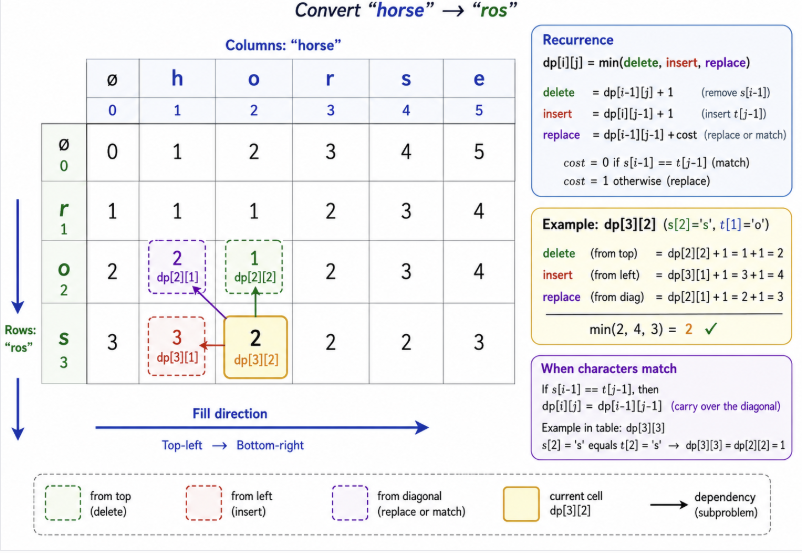
This recurrence has overlapping subproblems, so instead of recomputing the same values, we fill a dynamic programming table once and reuse the results.

For example, here is the table for "horse" and "ros":

The Input and the Pattern

To talk about the automaton, we need two strings:

• The pattern, $P$: the fixed string we are matching against. In the opening example, this is the query "resturants".
• The input, $I$: the candidate string we compare to the pattern, such as a dictionary word, restaurant name, or DNA sequence.

The asymmetry matters. Usually we have one query and many candidates. Since $P$ is fixed, we can build a machine specialized for it once, then run each input $I$ through that machine cheaply.

A Quick Detour: What Is an Automaton?

An automaton is an abstract machine that reads input one symbol at a time. The kind we need is a finite-state machine: it sits in one of a finite number of states, reads a symbol, and follows a transition to the next state. Some states are accepting. If the machine finishes the input in one of those states, it accepts the input.

For us, "accept" means "this input is within the allowed number of edits of the pattern." You can picture the machine as a graph of states and transitions, or implement it as a table where each state/input-symbol pair points to the next state.

Representing the Automaton as a DFA

We'll build a DFA (deterministic finite automaton), meaning that from any state, a given input character leads to exactly one next state. No guessing, no branching: one character in, one transition out.

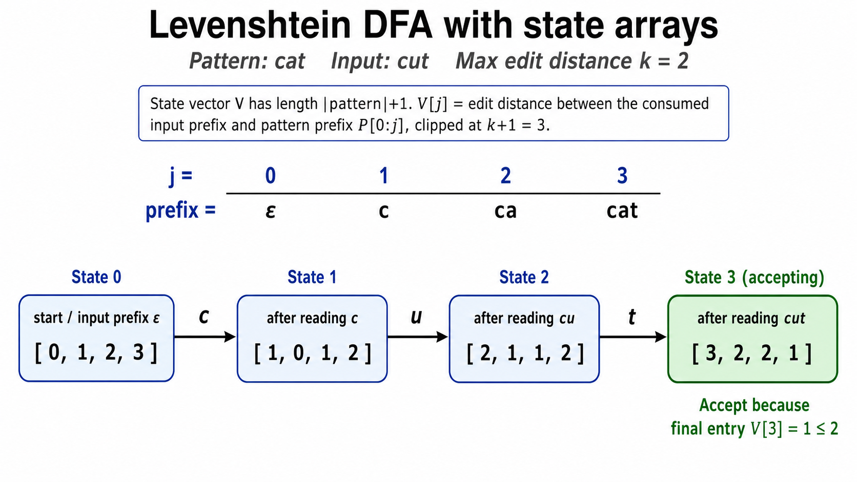
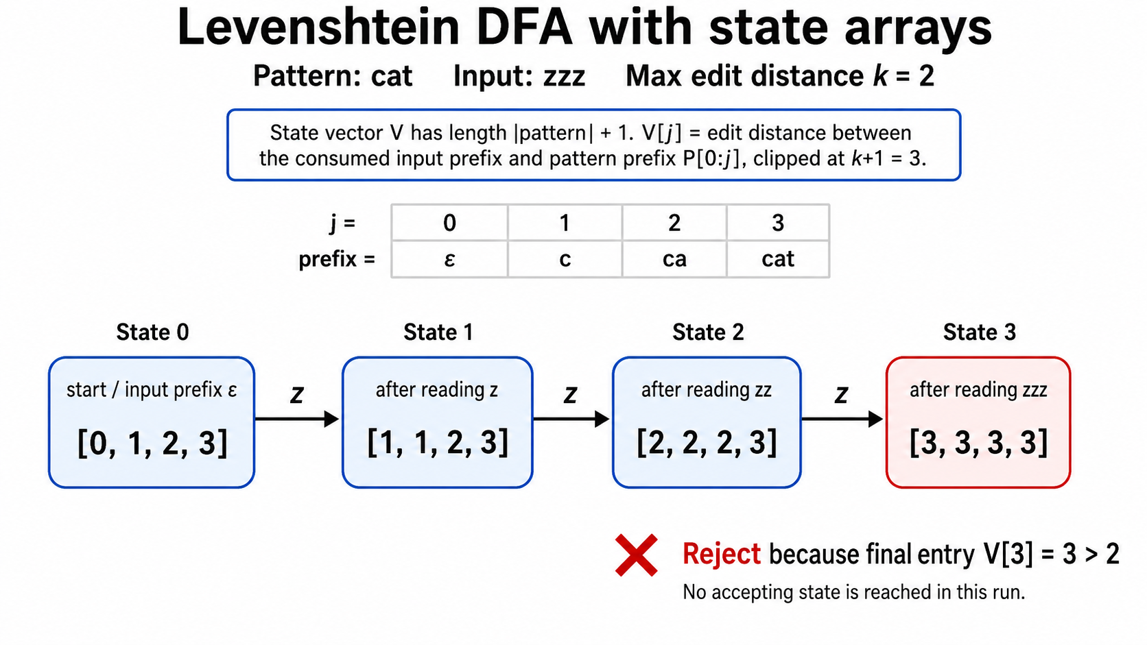
The key question is what a single state should remember. Look back at the DP table for "horse" and "ros". Each column corresponds to a prefix of the pattern $P$, including the empty prefix on the left. A single row of that table tells us, for every pattern prefix, the edit distance between that prefix and the part of the input we've read so far. That row is exactly the information a state needs to carry.

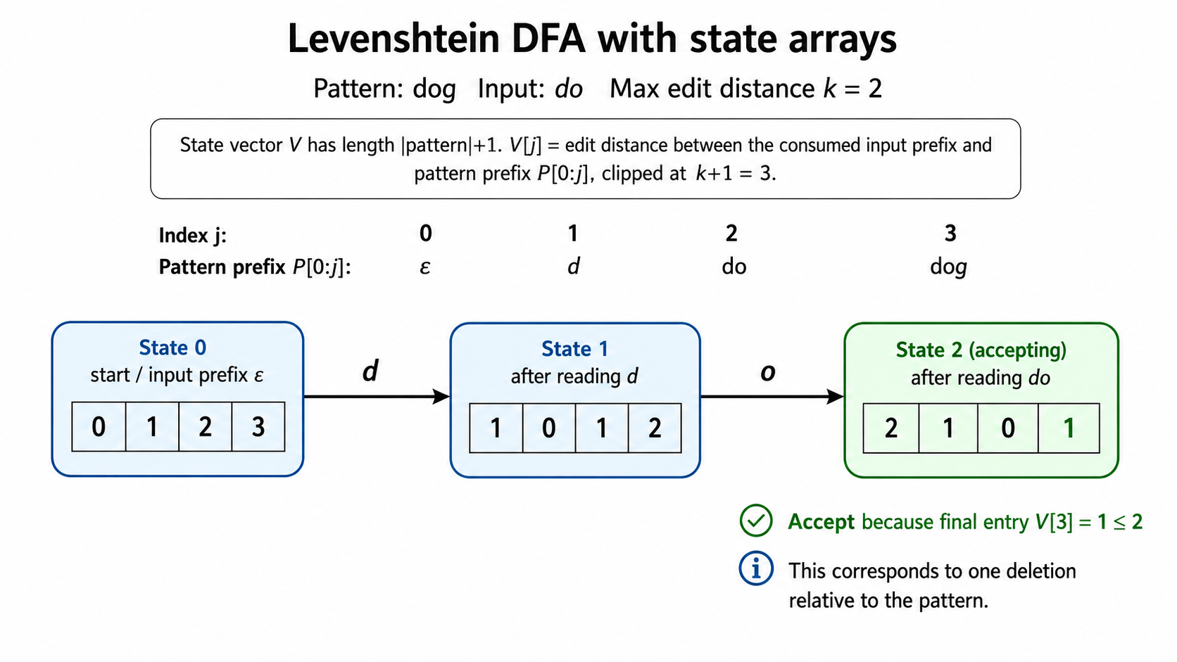
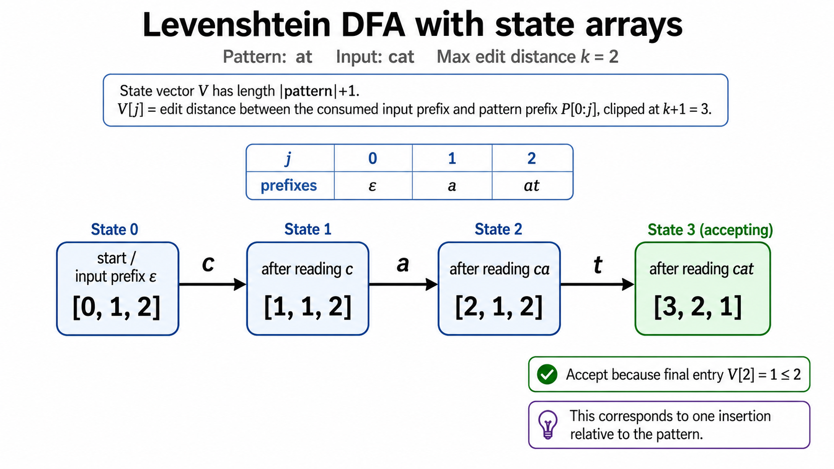
So a state is a vector of edit distances, one entry per prefix of $P$ (from the empty prefix up to the full pattern). But edit distances can grow without bound, which would give us infinitely many possible states. We fix this by choosing a maximum edit distance $K$ and clamping every entry to the range $0$ to $K + 1$, where $K + 1$ means "too far, gave up." With bounded values, the number of possible states becomes finite.

Transitions happen on characters of the input $I$. Each input character transforms one row of the DP table into the next row. A state summarizes "here is how far every prefix of $P$ is from the input prefix I've read so far," and each new character advances that summary by one step.

An input is accepted once the entry for the full pattern sits at $K$ or below: that's precisely the case where the whole pattern is within our edit budget of the input we've consumed.

The figures below show four short runs. Each is a single path through the DFA, not the whole transition graph: a substitution, a deletion relative to the pattern, an insertion relative to the pattern, and a rejected input.

How Many States Are There?

For the automaton to be practical, there had better not be too many states.

Recall that a state is a vector of $|P| + 1$ entries, one per prefix of $P$, each clamped to ${0, 1, \dots, K+1}$. Counting all such vectors naively gives

$$(K + 2)^{|P| + 1}$$

which is exponential in the pattern length and clearly hopeless. Almost none of those vectors can actually occur.

The first constraint is the staircase property: neighboring entries differ by at most 1, because extending a prefix by one character can change edit distance by at most one.

The second constraint is saturation. Edit distance is at least the difference in lengths:

$$D(i, j) \ge |,i - j,|$$

since each insertion or deletion changes the length by one. In the state reached after reading $i$ input characters, any cell with $|i - j| > K$ already exceeds our budget and saturates to $K + 1$.

So what is the widest non-saturated region a reachable vector can have? Think of the most spread-out valley possible. It starts at $K + 1$, descends one step at a time until it reaches 0, then climbs one step at a time back toward $K + 1$. The entries below saturation are

$$K, K-1, \dots, 0, \dots, K-1, K$$

which gives a maximum width of $2K + 1$ interesting entries. For example, when $K = 1$, entries range from 0 to 2, and the widest valley looks like

$$2,\ 1,\ 0,\ 1,\ 2,\ 2,\ 2,\ \dots$$

Only the middle three entries are below the saturated value 2. Everything outside the valley is flat at $K + 1$ and carries no extra information.

That gives us a sharper way to count possible state shapes. A non-saturated region has at most $2K + 1$ entries. Its shape is determined by:

• The first value, which can be any value from $0$ to $K + 1$, giving $K + 2$ choices.
• Each following step, which can go down, stay flat, or go up, giving 3 choices for each of the remaining $2K$ entries.

Multiplying the two gives

$$
(K + 2)\cdot 3^{2K}
$$

possible shapes per band position. There are $O(|P| + 1)$ places where that band can sit, so the total number of reachable states is bounded by

$$
O\big((|P| + 1)\cdot(K + 2)\cdot 3^{2K}\big).
$$

The important part is not the exact constant. For a fixed band position, the number of possible state shapes depends only on $K$, not on $|P|$; the pattern length only decides how many places that bounded window can sit. Since $K$ is usually 1 or 2 in fuzzy-search applications, the total number of states grows effectively linearly with $|P|$.

Runtime

Keep two costs separate: building the automaton once, and running inputs through it many times.

Running an input is the payoff. Once the transition table exists, matching $I$ is just a walk over the DFA: read a character, follow one transition, repeat. Each transition is a constant-time lookup, so a full match is $O(|I|)$, independent of the pattern length and of $K$ at query time. Recomputing edit distance from scratch would cost $O(|P| \cdot |I|)$ for every candidate.

Building the automaton costs on the order of the number of states and transitions. If $S$ is the number of reachable states, the table has $O(S \cdot |\Sigma|)$ entries, one transition per state and alphabet symbol. Using the bound above, that is $O((|P| + 1)\cdot(K + 2)\cdot 3^{2K}\cdot|\Sigma|)$ table entries.

The trade is: spend more up front for a fixed pattern, then make every input afterward cheap. If you compute transitions on the fly instead of precomputing them, each step costs $O(K)$ with a banded update.

A Reference Implementation

I wrote a working implementation in Rust at galsterGH/levenshtein-automaton. A state is the vector of edit distances we've been drawing, Vec<usize>, with every entry clamped to diffs_allowed + 1. The initial state is the first DP row: edit_distance[i] = min(i, diffs_allowed + 1).

Construction is a breadth-first search from that initial state. For each state, the implementation computes its transition on every alphabet character, deduplicates identical rows with a HashMap, and stops expanding dead states. Matching a word is then the cheap walk from earlier: consume characters, follow transitions, and check whether the final state is accepting.

The repo also pairs the automaton with a Trie for dictionary search. The Matcher walks the Trie and DFA together, pruning an entire Trie subtree as soon as the automaton reaches a dead state.

Wrapping Up

We started with a simple question: how do you find strings that are close but not identical? The path was:

• Edit distance measures similarity as the minimum number of insertions, deletions, and substitutions between two strings.
• Fixing the pattern $P$ and streaming the input $I$ turns one row of the DP table into a state of a DFA.
• Clamping distances to $K + 1$ and noticing that only a diagonal band matters keeps the automaton small for the small values of $K$ used in practice.
• That small automaton, built once, matches any input in $O(|I|)$, independent of the pattern length, and pairs naturally with a Trie to fuzzy-search an entire dictionary.

What I find beautiful about the Levenshtein automaton is that it is really just the edit-distance table seen from another angle. The recurrence did not change. We only noticed that one string stays fixed, and after precomputing for that string, an $O(|P| \cdot |I|)$ comparison becomes an $O(|I|)$ lookup. It is a good reminder to ask: what here is actually fixed, and what am I recomputing as if it were not?